根据B站视频整理的笔记,看完基本可以入门Pytorch。
1 环境配置 conda 技巧pip 安装Pytorch 检验安装 2 编辑器的选择 PyCharm 配置PyCharm 一些技巧 Jupyter jupyter 配置 3 Python的两大法宝函数 4 浅对比PyCharm,python控制台和Jupyter 5 PyTorch加载数据 提供不同的数据形式 5.1 TensorBoard的使用 SummaryWriter writer.add_scalar() 效果 writer.add_image() writer.add_graph(net,input) 5.2 Transform ToTensor 归一化Normalization Resize() Compose() RandomCrop()随机裁剪 总结 6 Torchvision的数据集使用 7 Dataloader的使用 8 网络搭建 8.1 Containers nn.Module 8.2 卷积层操作与卷积层 (1)卷积操作 基本原理 (2)卷积层 8.3 池化 特征 8.4 非线性激活 (1) ReLu(Rectified Linear Unit) (2)Sigmoid 8.5 Linear model 9 损失函数与反向传播 损失函数 反向传播 10 优化器 SGD随机梯度下降 11 现有网络模型的使用和修改 11.1 VGG简介 利用现有的网络,套到自己的数据集上 12 网络模型的保存与读取 12.1 保存模型与参数 12.2 保存模型参数 12 完整模型训练套路 13 使用GPU训练 13.1 13.2 14 完整模型验证套路 15 Github开源代码 1 环境配置
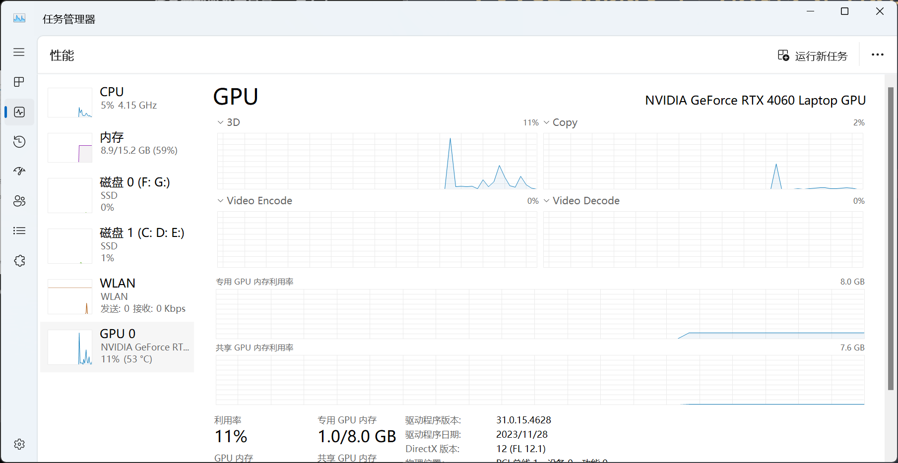
检查显卡:
conda
#conda
1 conda create -n [env name] python=[python version]
1 conda activate [env name]
技巧pip
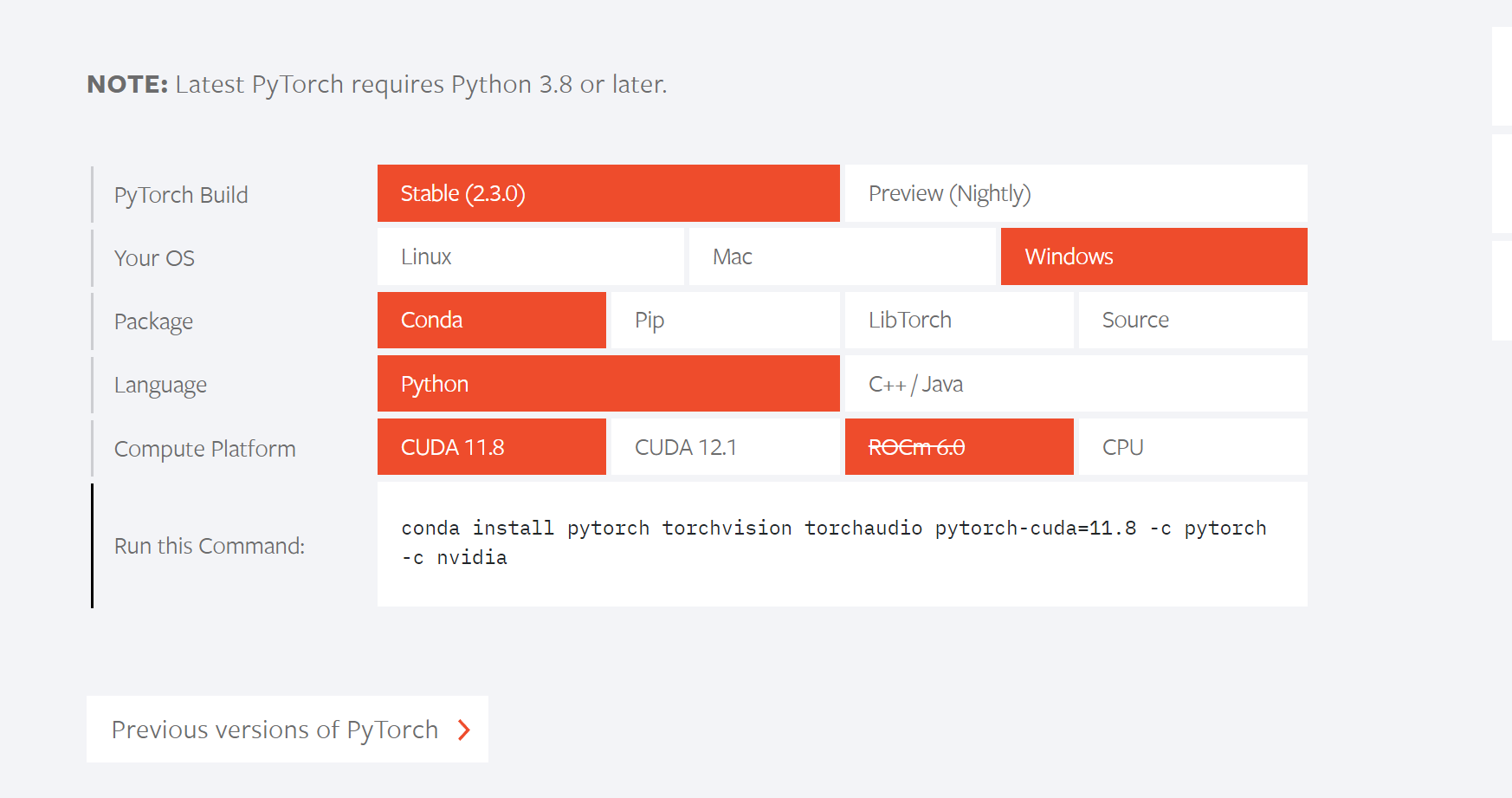
安装Pytorch
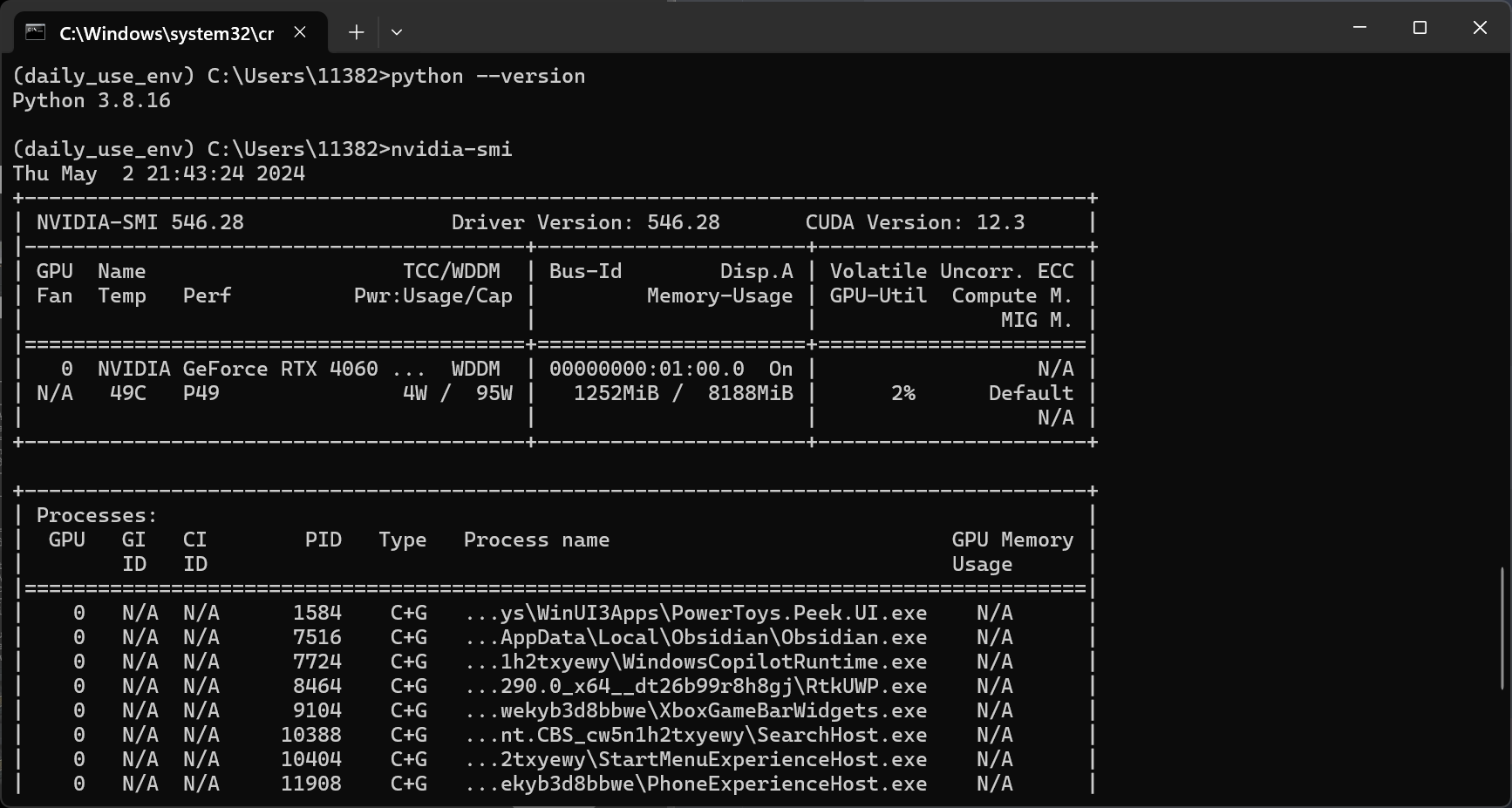
检查电脑的GPU是否支持pytorchnvidia-smi
查看驱动版本 Driver Version
需要保持版本号大于coda的需求的
如果不满足,可以去英伟达的官网 更新驱动
选好后,输入conda命令即可
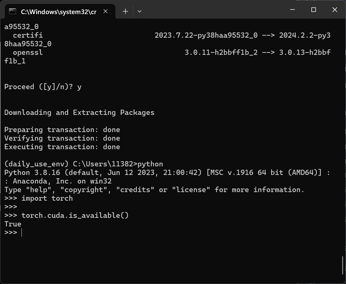
检验安装
1
2
3
>>python >>import torch # 没有报错就是安装成功 >>torch.cuda.is_available() # 检查是否可以使用GPU
torch.cuda.is_available()返回False
进入https://www.nvidia.cn/geforce/technologies/cuda/supported-gpus/
检查是否支持cuda
检查驱动版本nvidia-smi
不够高就去更新
在正常使用一段时间后,安装各种包突然又返回False或者各种冲突。
卸载torch全部重来:conda remove pytorch torchvision
2 编辑器的选择
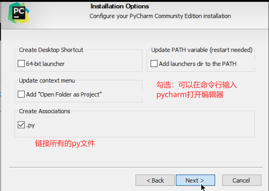
PyCharm
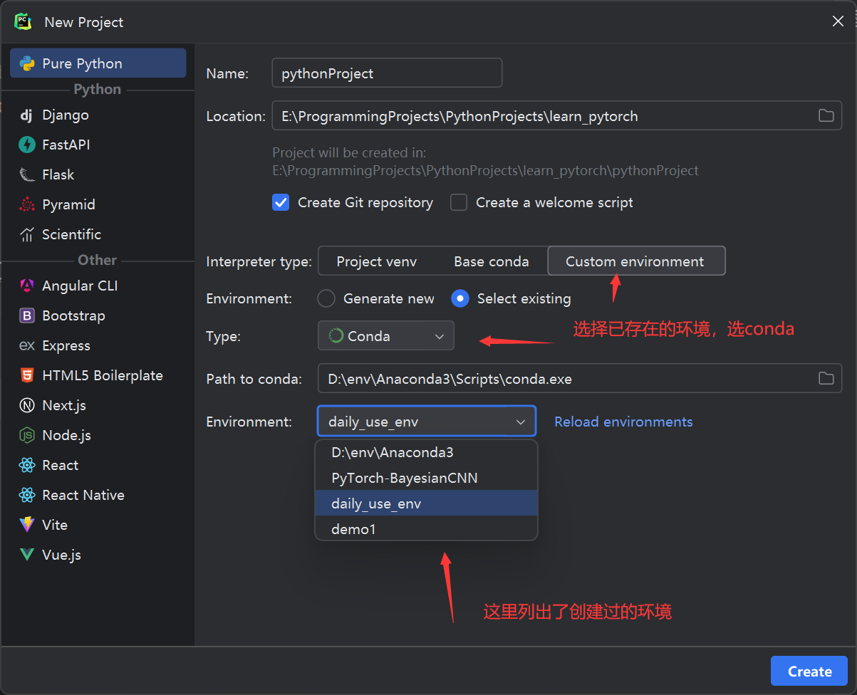
配置PyCharm
一些技巧
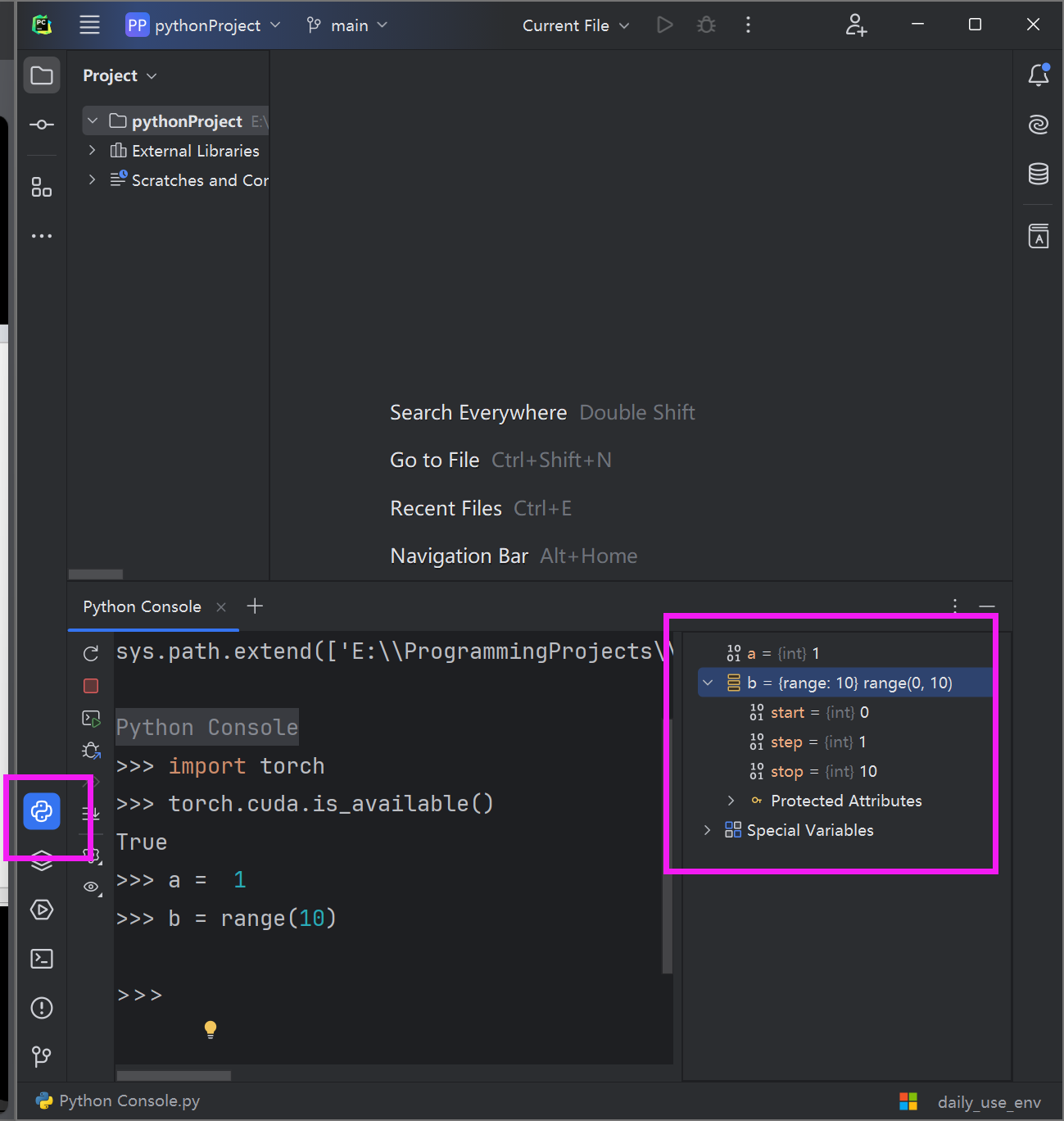
python的console,可以检查一些变量或者一些命令、方法,简便直观。
Jupyter
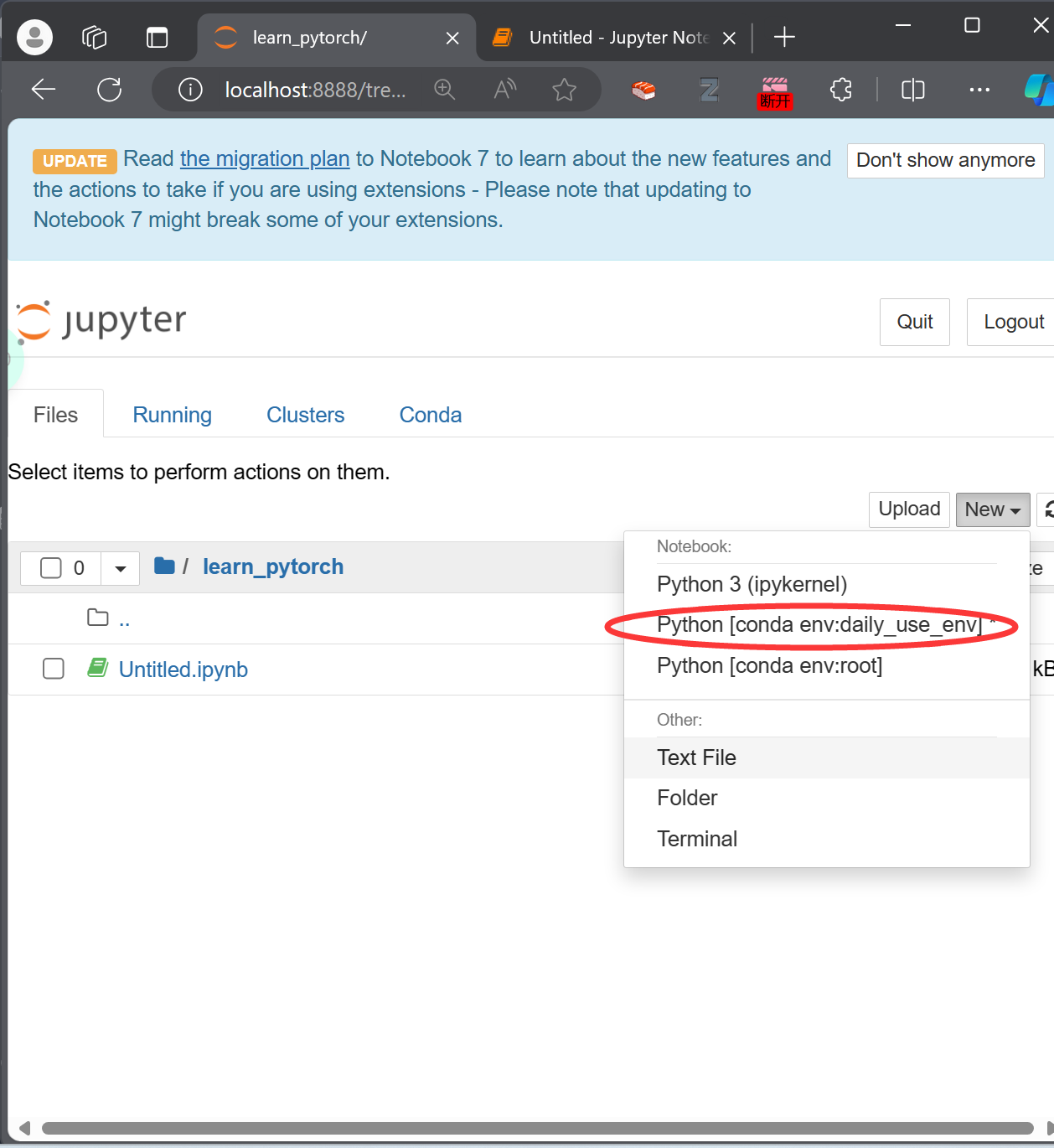
jupyter 配置
在安装cuda的时候,这个默认安装在base的环境中。但是base中没有安装torch。可以再在base里面安装一次torch,但是还是在之前安装的torch环境中安装一下jupyter吧~
安装一个个包nb_conda 是一个用于 Jupyter Notebook 的插件,它可以让你在 Notebook 中使用 Conda 环境。通过运行 conda install nb_conda,你可以将这个插件安装到你的 Conda 环境中,然后在 Jupyter Notebook 中使用。这样你就可以方便地在 Notebook 中管理和切换不同的 Conda 环境了。
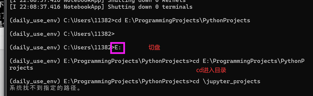
在命令行中切换到对应的项目目录
创建项目
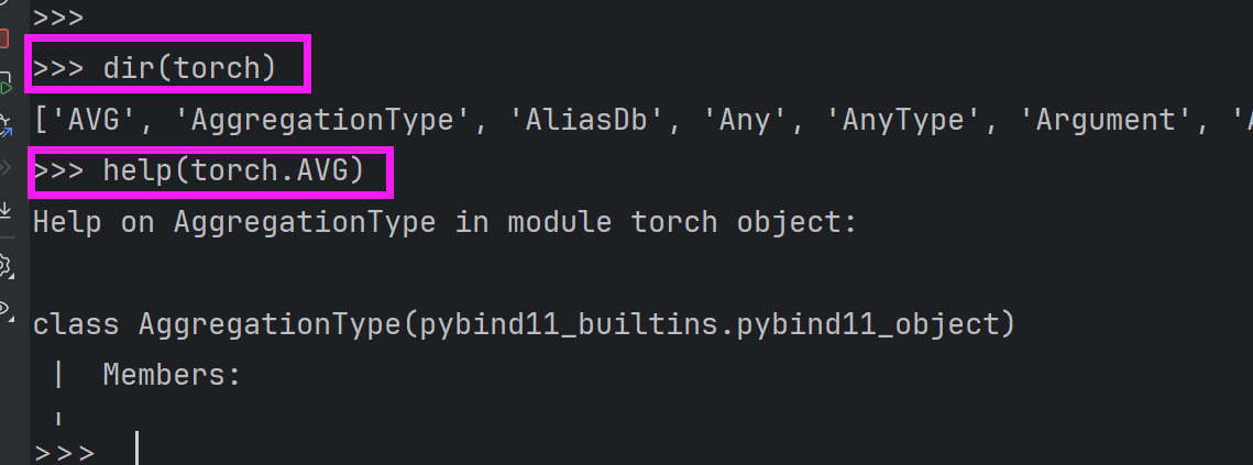
3 Python的两大法宝函数
4 浅对比PyCharm,python控制台和Jupyter
rerun的区别
PyCharm会全部重新运行。
控制台:从错误的地方开始运行
notebook:任意行为块,每一块重运行。
5 PyTorch加载数据
Dataset:
获取的数据是混乱的,但是可以进行编号
可以获取数据和label
Dataloader:
#os的用法
os.path.join(dir1,dir2):可以根据系统自动拼接地址
1
2
3
4
5
6
7
8
9
10
11
12
13
14
15
16
17
18
19
20
21
22
23
24
25
26
27
28
29
30
31
32
33
34
35
36
37
38
''' @Project :pythonProject @File :read_data.py @IDE :PyCharm @Author :周大猛 @Date :2024/05/02 23:50 ''' from torch.utils.data import Dataset from PIL import Image import os class MyDataset (Dataset ): def __init__ (self, root_dir, label_dir ): self.root_dir = root_dir self.label_dir = label_dir self.path = os.path.join(root_dir, label_dir) self.img_path = os.listdir(self.path) def __getitem__ (self, index ): """ 读取每一个图片 :param index: :return: """ img_name = self.img_path[index] img_item_path = os.path.join(self.path, img_name) img = Image.open (img_item_path) label = self.label_dir return img, label def __len__ (self ): """获得数据集的长度""" return len (self.img_path) if __name__ == '__main__' : root_dir = "dataset/train" ants_label_dir = "ants" bees_label_dir = "bees" ants_dataset = MyDataset(root_dir,ants_label_dir) bees_dataset = MyDataset(root_dir,bees_label_dir) train_loader = ants_dataset + bees_dataset
5.1 TensorBoard的使用
SummaryWriter
原文部分介绍:
1
2
3
4
5
6
7
8
9
10
11
12
13
14
15
16
17
18
19
20
21
22
class SummaryWriter : """Writes entries directly to event files in the log_dir to be consumed by TensorBoard. The `SummaryWriter` class provides a high-level API to create an event file in a given directory and add summaries and events to it. The class updates the file contents asynchronously. This allows a training program to call methods to add data to the file directly from the training loop, without slowing down training. """ def __init__ ( self, log_dir=None , comment="" , purge_step=None , max_queue=10 , flush_secs=120 , filename_suffix="" , ): """Create a `SummaryWriter` that will write out events and summaries to the event file. Args: log_dir (str): Save directory location. Default is runs/**CURRENT_DATETIME_HOSTNAME**, which changes after each run. Use hierarchical folder structure to compare between runs easily. e.g. pass in 'runs/exp1', 'runs/exp2', etc. for each new experiment to compare across them. comment (str): Comment log_dir suffix appended to the default ``log_dir``. If ``log_dir`` is assigned, this argument has no effect. purge_step (int): When logging crashes at step :math:`T+X` and restarts at step :math:`T`, any events whose global_step larger or equal to :math:`T` will be purged and hidden from TensorBoard. Note that crashed and resumed experiments should have the same ``log_dir``. max_queue (int): Size of the queue for pending events and summaries before one of the 'add' calls forces a flush to disk. Default is ten items. flush_secs (int): How often, in seconds, to flush the pending events and summaries to disk. Default is every two minutes. filename_suffix (str): Suffix added to all event filenames in the log_dir directory. More details on filename construction in tensorboard.summary.writer.event_file_writer.EventFileWriter. Examples:: from torch.utils.tensorboard import SummaryWriter # create a summary writer with automatically generated folder name. writer = SummaryWriter() # folder location: runs/May04_22-14-54_s-MacBook-Pro.local/ # create a summary writer using the specified folder name. writer = SummaryWriter("my_experiment") # folder location: my_experiment # create a summary writer with comment appended. writer = SummaryWriter(comment="LR_0.1_BATCH_16") # folder location: runs/May04_22-14-54_s-MacBook-Pro.localLR_0.1_BATCH_16/ """
三种用法
默认保存到一个路径 writer = SummaryWriter() # folder location: runs/May04_22-14-54_s-MacBook-Pro.local/
自定义保存到的文件夹 writer = SummaryWriter("my_experiment") # folder location: my_experiment
可以对文件名加入一些comments writer = SummaryWriter(comment="LR_0.1_BATCH_16") # folder location: runs/May04_22-14-54_s-MacBook-Pro.localLR_0.1_BATCH_16/
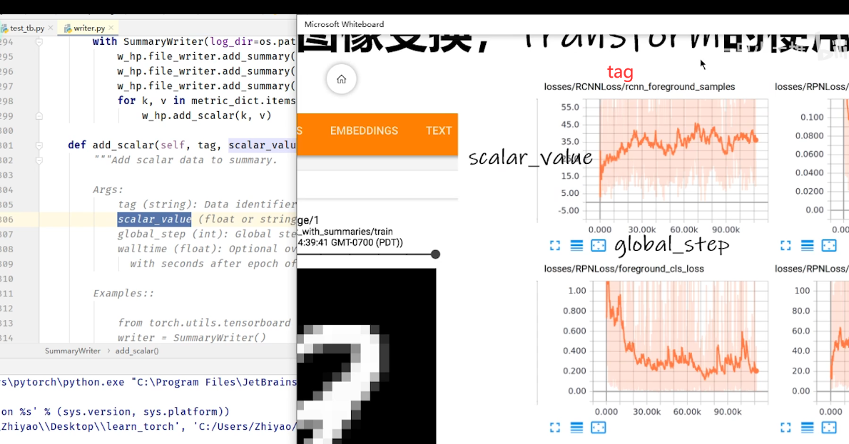
writer.add_scalar()
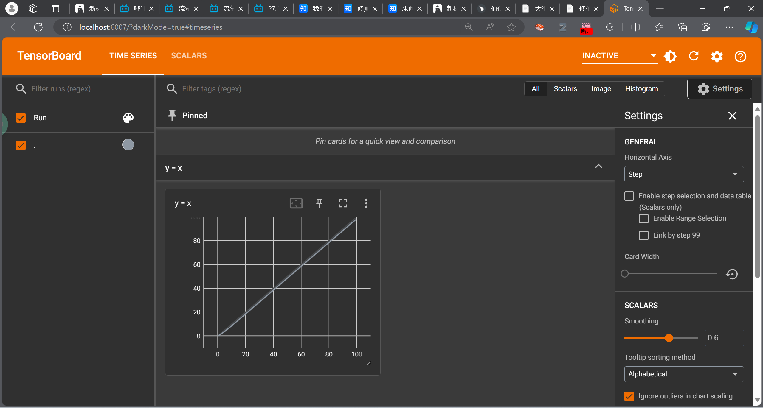
效果
打开方法:
指定路径 --logdir
指定端口 --port
1 tensorboard --logdir=[logs] --port=[6007]
但是运行多次之后可能显示图像会出bug,可以选择删掉之前的log
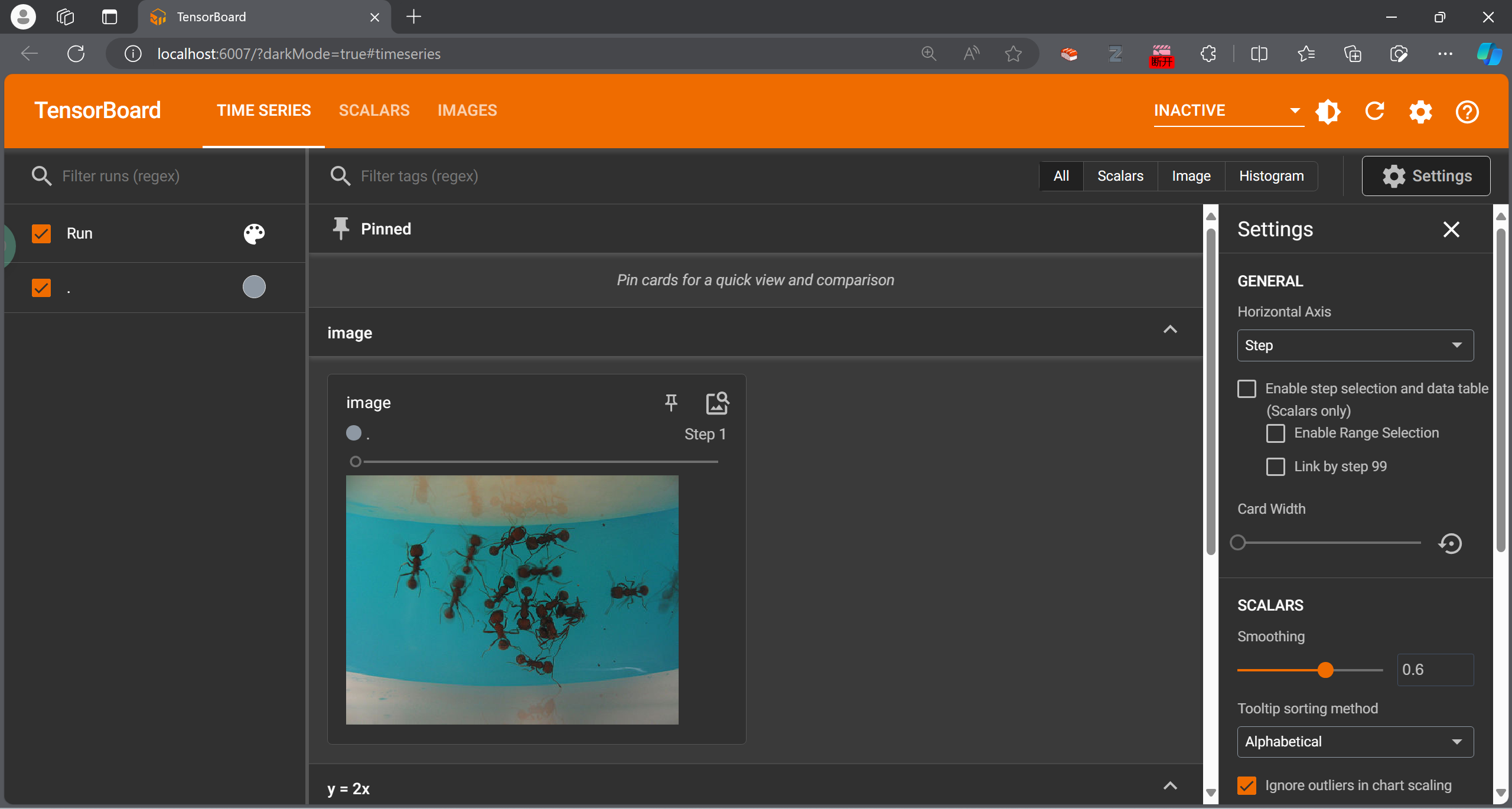
writer.add_image()
但是我们常用的PIL的Image是JpegImageFile类型,所以不符合,需要转换,或者直接用别的方法读取图片,如OpenCV
在使用numpy读取图片的时候,每个通道的顺序可能与add_image默认的顺序不一样,可以ctrl进入add_image查看手册,手动设定通道顺序
1
2
3
4
5
6
7
8
9
10
11
from PIL import Image from torch.utils.tensorboard import SummaryWriter import numpy as np writer = SummaryWriter('logs' ) image_path = "dataset/train/ants/5650366_e22b7e1065.jpg" iamge_PIL = Image.open (image_path) img_array = np.array(iamge_PIL) print (img_array.shape) writer.add_image("image" , img_array, 1 ,dataformats='HWC' )
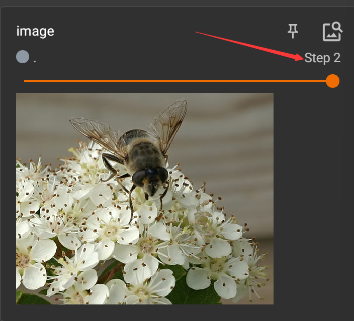
修改add_image的第二个参数step,可以在进度条处出现拉出新的图
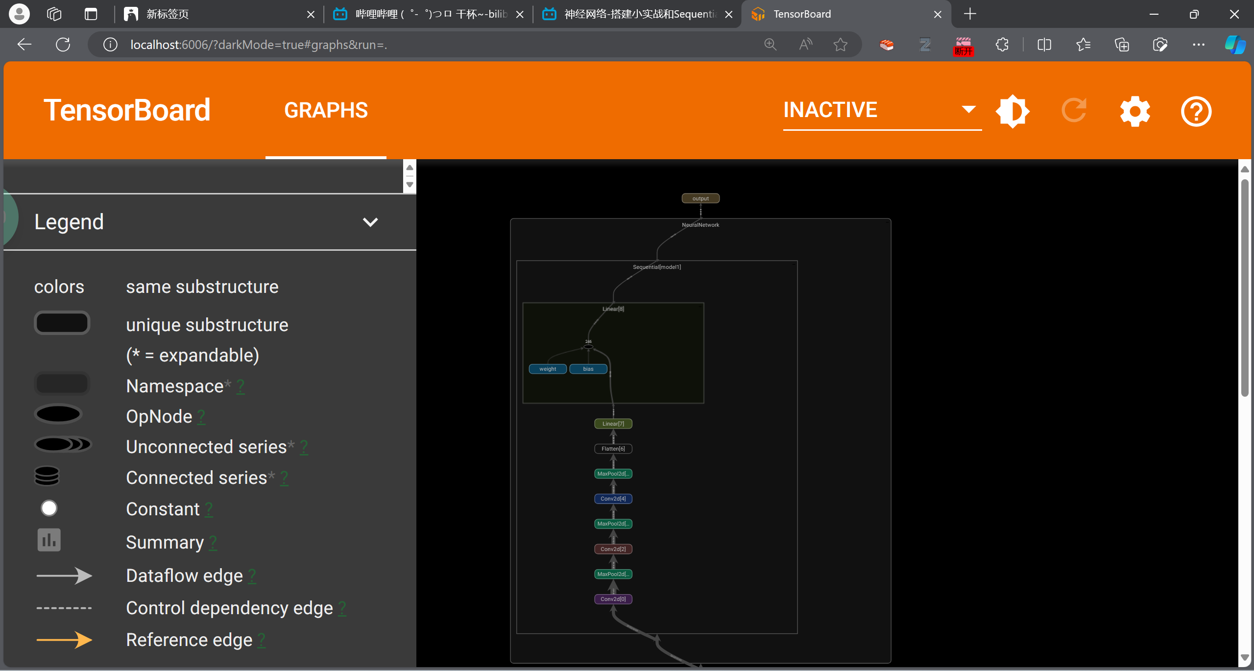
可以查看网络的结构
1 2 3 4 writer = SummaryWriter("./logs" ) writer.add_graph(net,input ) writer.close()
指的是:transforms.py文件,里面又很多的“工具”:
拿特定格式的图片,丢进去,得到需要的图片结果。
引入的方式
1 from torchvision import transforms
ToTensor
1
2
tensor_trans = transforms.ToTensor() tensor_img = tensor_trans(image)
为什么需要Tensor这个数据类型?
另一种读取方式:nparray
导入opencv的方法:
1 pip install opencv-python
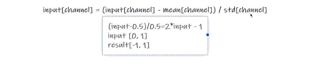
归一化Normalization
output[channel] = (input[channel] - mean[channel]) / std[channel]
均值和标准差都是0.5
1
2
3
4
trans_norm = transforms.Normalize([0.5 ,0.5 ,0.5 ], [0.5 ,0.5 ,0.5 ]) img_norm = trans_norm(img_tensor) writer.add_image('Normal_img' , img_norm)
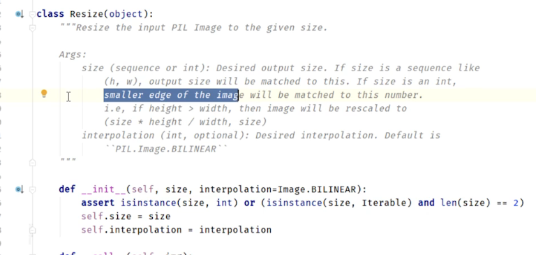
Resize()
1 2 3 4 5 6 7 8 9 10 print (img.size) trans_resize = transforms.Resize((512 ,512 )) img_resize = trans_resize(img) img_resize = trans_totensor(img_resize) writer.add_image('Resize_img' , img_resize,0 ) print (img_resize) writer.close()
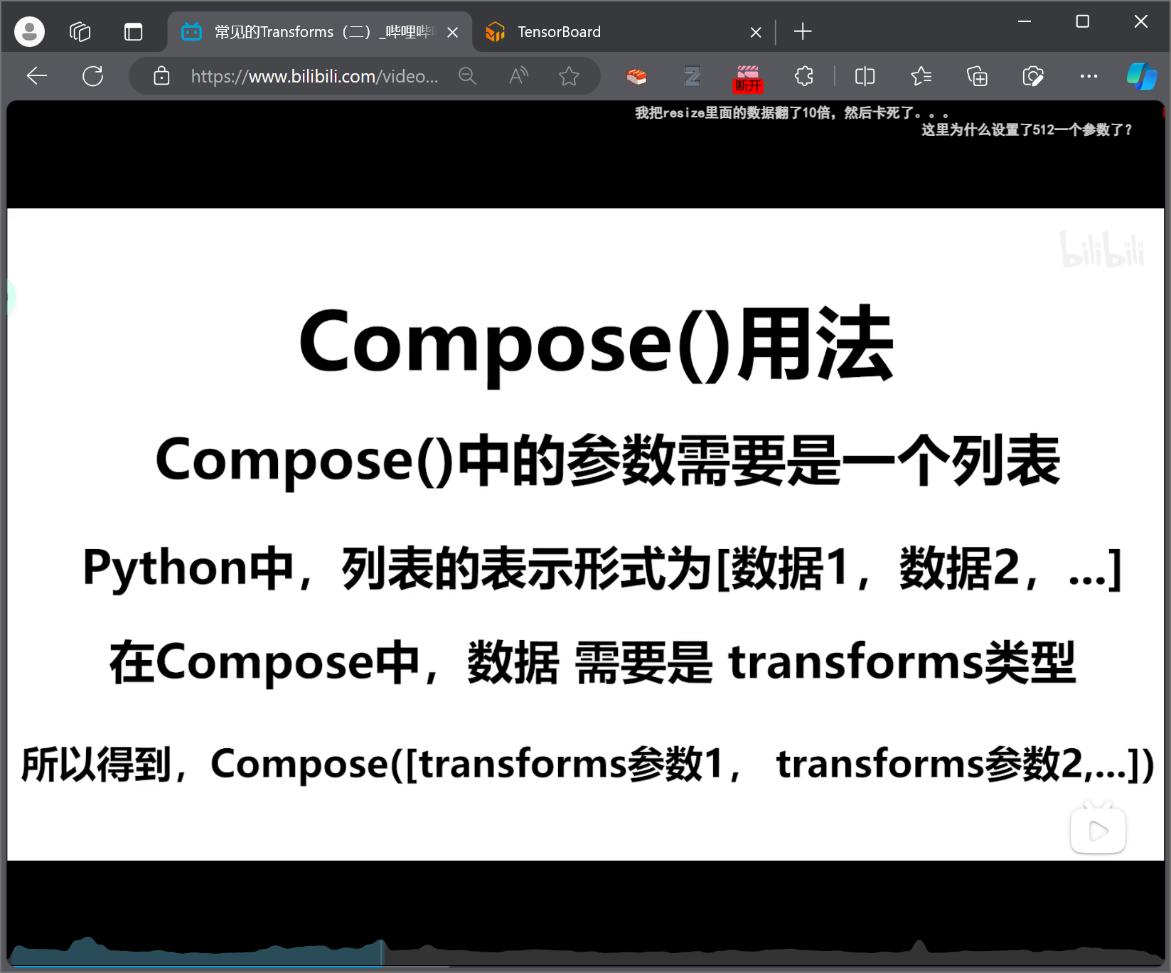
Compose()
1 2 3 4 5 6 trans_resize_2 = transforms.Resize(64 ) trans_compose = transforms.Compose([trans_resize_2,trans_totensor,]) img_resize_2 = trans_compose(img)
RandomCrop()随机裁剪
按照设定的尺寸随机在图片内裁剪规定尺寸大小的图片。
1 2 3 4 5 6 trans_random = transforms.RandomCrop(64 ) trans_compose_2 = transforms.Compose([trans_random,trans_totensor,]) for i in range (10 ): img_crop = trans_compose_2(img) writer.add_image('Random_img' , img_crop,i)
总结
关注输入和输出的类型
多看官方文档
看初始化的参数
输出类型可以print查看,或者debug
6 Torchvision的数据集使用
官网链接
如果下载速度太慢,可以将下载路径粘贴到迅雷中进行下载。
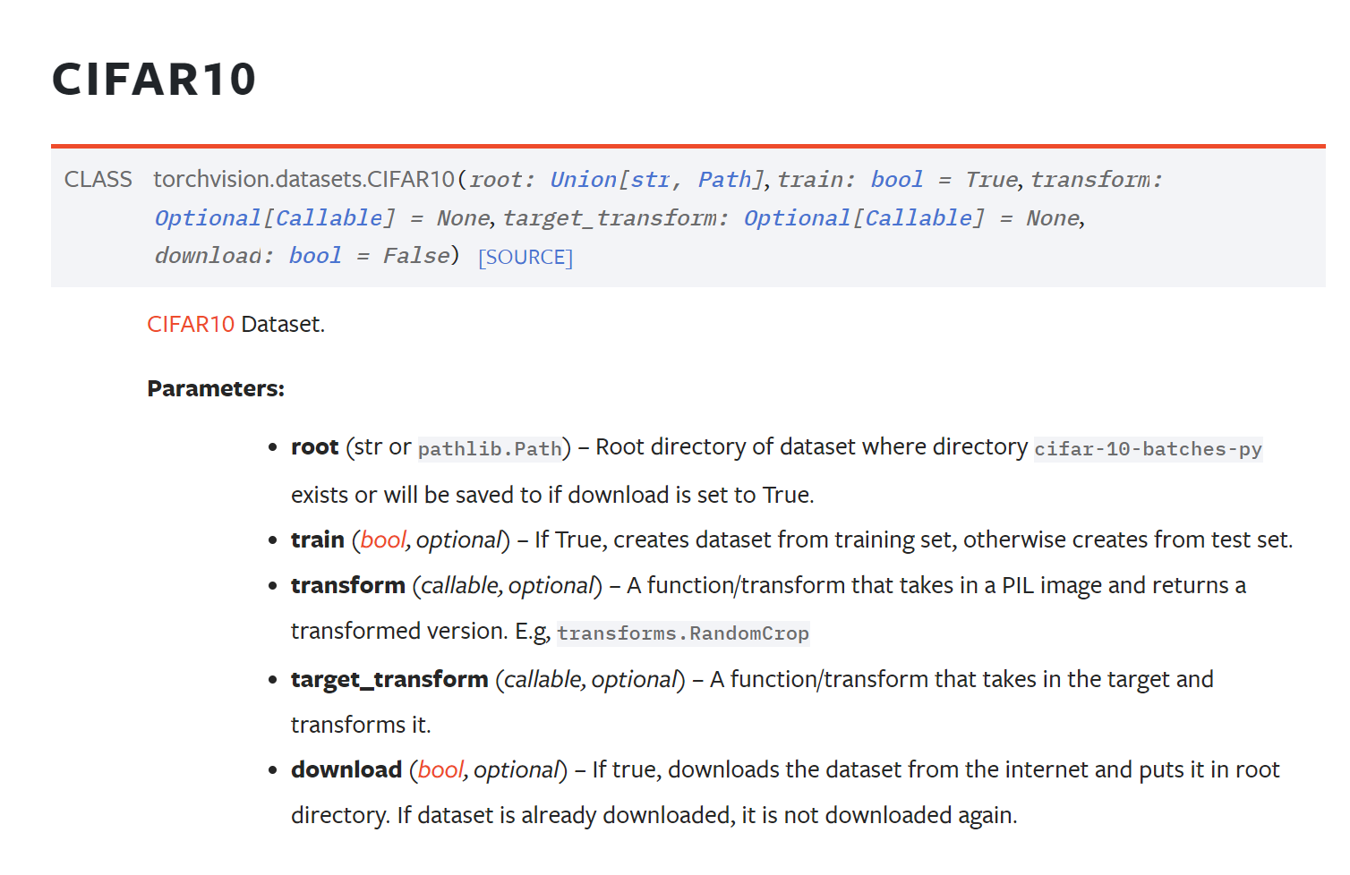
数据集的参数设置很多都是相同的,教程中以CIFAR10为例:
设置数据集路径
设置训练or测试集合
transform要做的操作
download:是否要网络下载(准备好了就False,没准备就True)
1
2
3
4
import torchvision train_set = torchvision.datasets.CIFAR10(root='./data' , train=True , download=True ) test_set = torchvision.datasets.CIFAR10(root='./data' , train=False , download=True )
可以在transform参数,设置对数据集的操作,也是可以打包送进去的。
1
2
3
4
5
6
7
8
9
10
11
12
13
14
15
16
17
18
19
20
21
import torchvision from torch.utils.tensorboard import SummaryWriter dataset_transform = torchvision.transforms.Compose([ torchvision.transforms.ToTensor(), torchvision.transforms.Normalize(mean=[0.485 , 0.456 , 0.406 ], std=[0.229 , 0.224 , 0.225 ]), ]) train_set = torchvision.datasets.CIFAR10(root='./data' , train=True , download=True , transform=dataset_transform) test_set = torchvision.datasets.CIFAR10(root='./data' , train=False , download=True , transform=dataset_transform) print (test_set[0 ]) writer = SummaryWriter(log_dir='./logs' ) for i in range (10 ): img, label = test_set[i] writer.add_image('test_img' , img, i)
7 Dataloader的使用
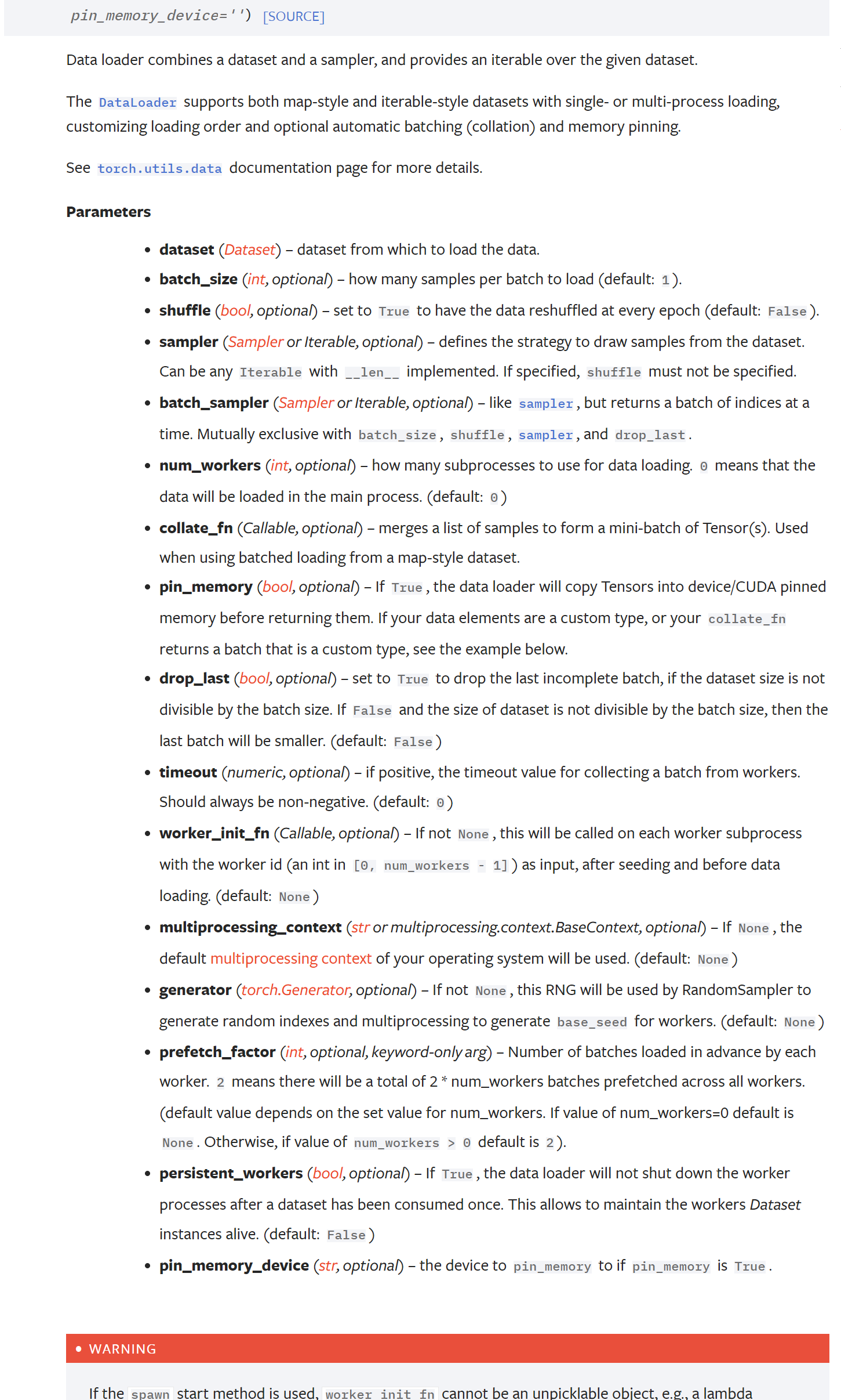
将数据加载到神经网络中。
如何取 数据可以由Dataloader进行设置。
常用参数设置:
batch_size
shuffle:洗牌
num_workers:多少个进行进行加载(但是win上有时候出现错误)
drop_last:分组除不尽的时是否舍去一些数据。
DataLoader会分别把数据集的数据和label,按照batch_size的大小,进行打包。
如果设置了shuffle,一个epoch打乱一次。
1
2
3
4
5
6
7
8
9
10
11
12
13
14
15
16
17
18
19
20
21
22
23
24
25
26
27
28
import torchvision from torch.utils.data import DataLoader from torch.utils.tensorboard import SummaryWriter from torchvision import transforms data_transforms = transforms.Compose([transforms.ToTensor(),]) test_data = torchvision.datasets.CIFAR10(root='./data' , train=False , download=True ,transform=data_transforms) test_loader = DataLoader(dataset=test_data, batch_size=64 , shuffle=True ,num_workers=0 , drop_last=False ) img, label = test_data[0 ] print (img.shape) print (label) writer = SummaryWriter('./logs' ) for epoch in range (10 ): step = 0 for data in test_loader: imgs, labels = data writer.add_images('Epoch:{}' .format (epoch), imgs,step) step += 1 writer.close()
8 网络搭建
https://pytorch.org/docs/stable/nn.html
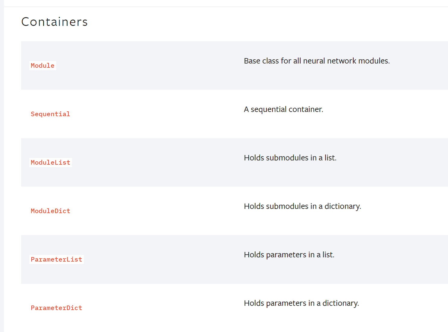
8.1 Containers
最常用的模块,提供神经网络的最基本的框架
nn.Module
》 https://pytorch.org/docs/stable/generated/torch.nn.Module.html#torch.nn.Module
1
2
3
4
5
6
7
8
9
10
11
12
13
14
15
import torch.nn as nnimport torch.nn.functional as Fclass Model (nn.Module): def __init__ (self ): super ().__init__() self.conv1 = nn.Conv2d(1 , 20 , 5 ) self.conv2 = nn.Conv2d(20 , 20 , 5 ) def forward (self, x ): x = F.relu(self.conv1(x)) return F.relu(self.conv2(x))
8.2 卷积层操作与卷积层
(1)卷积操作
基本原理
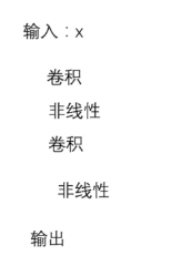
在全连接(Affine)层中存在忽略了数据形状,它直接将整个图片拉成一维数据输入到了神经网络。
因此导致了,形状中含有的空间信息被忽略。
卷积层的优点就是,可以保持形状的不变,或许能更好的理解图片的形状信息。
卷积层的输入输出被称为特征图 ,。
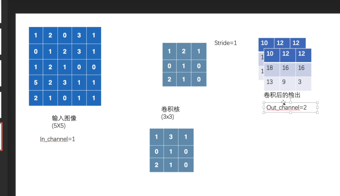
卷积核:(类似图像处理的滤波器)一个小矩阵,对图像矩阵进行一坨一坨的计算
stride = 滤波器每次移动的举例
会影响最后得到的卷积输出的形状
越大,输出的矩阵越小(?)
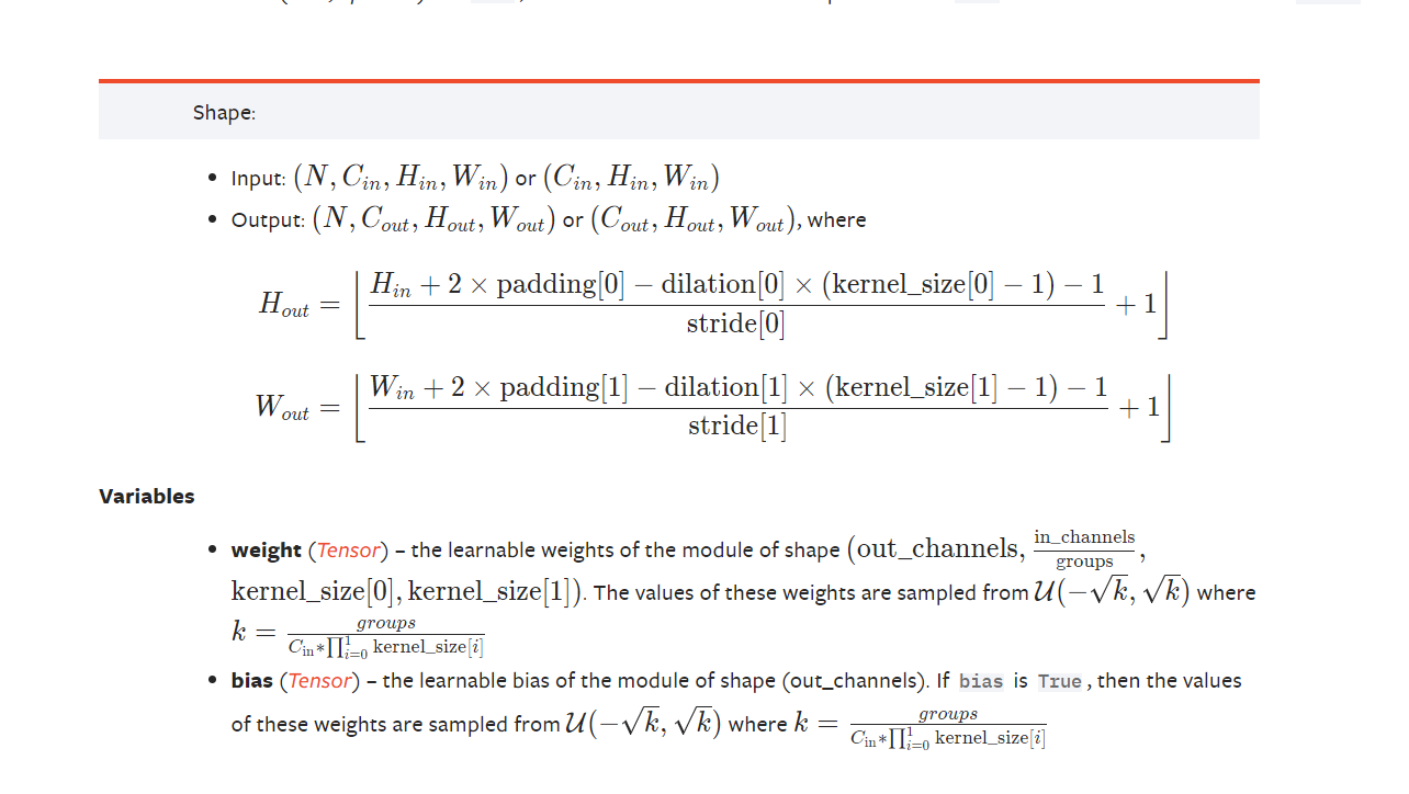
官网参数介绍:conv2d
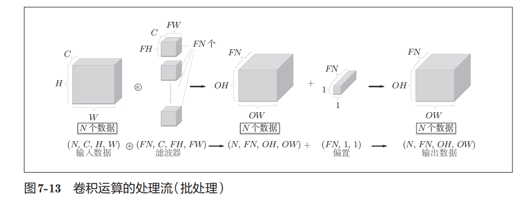
input – input tensor of shape (minibatch,in_channels,𝑖𝐻,𝑖𝑊)(minibatch,in_channels,iH,iW)
要设置batch的带线啊哦
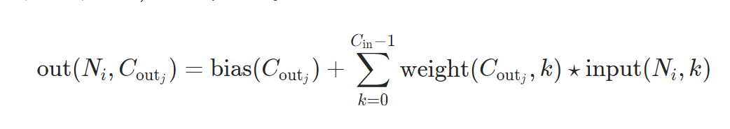
weight – filters of shape (out_channels,in_channelsgroups,𝑘𝐻,𝑘𝑊)(out_channels,groupsin_channels,kH,kW)
bias – optional bias tensor of shape (out_channels)(out_channels). Default: None
stride – the stride of the convolving kernel. Can be a single number or a tuple (sH, sW). Default: 1
padding (在图像左右两边对图像进行填充)–
implicit paddings on both sides of the input. Can be a string {‘valid’, ‘same’}, single number or a tuple (padH, padW). Default: 0 padding='valid' is the same as no padding. padding='same' pads the input so the output has the same shape as the input. However, this mode doesn’t support any stride values other than 1.
1
2
3
4
5
6
7
8
9
10
11
12
13
14
15
16
17
18
19
20
21
22
23
24
25
26
27
28
29
30
31
32
33
34
35
36
37
38
import torch import torch.nn.functional as F input = torch.tensor([[1 ,2 ,0 ,3 ,1 ], [0 ,1 ,2 ,3 ,1 ], [1 ,2 ,1 ,0 ,0 ], [5 ,2 ,3 ,1 ,1 ], [2 ,1 ,0 ,1 ,1 ]]) kernel = torch.tensor([[1 ,2 ,1 ], [0 ,1 ,0 ], [2 ,1 ,0 ]]) input = torch.reshape(input ,(1 ,1 ,5 ,5 )) kernel = torch.reshape(kernel,(1 ,1 ,3 ,3 )) output1 = F.conv2d(input ,kernel,stride=1 ) print (output1) output2 = F.conv2d(input ,kernel,stride=2 ) print (output2) output3 = F.conv2d(input ,kernel,stride=1 ,padding=1 ) print (output3)
(2)卷积层
https://pytorch.org/docs/stable/generated/torch.nn.Conv2d.html#torch.nn.Conv2d
Parameters
in_channels (int
out_channels (int
kernel_size (int or tuple
stride (int or tuple , optional ) – Stride of the convolution. Default: 1
padding (int , tuple or str , optional ) – Padding added to all four sides of the input. Default: 0
padding_mode (str , optional ) – 'zeros', 'reflect', 'replicate' or 'circular'. Default: 'zeros'
dilation (int or tuple , optional ) – Spacing between kernel elements. Default: 1
groups (int , optional ) – Number of blocked connections from input channels to output channels. Default: 1
bias (bool , optional ) – If True, adds a learnable bias to the output. Default: True
根据这两个公式,推到论文中的padding和stride
#padding计算 #stride计算
#批处理
8.3 池化
#池化
特征
无需学习参数(与卷积的不同)
通道数不发生变化
对微笑的数据位置变化具有鲁棒性(健壮)
Parameters
kernel_size (Union [ int , Tuple [ int , int ]__] ) – the size of the window to take a max over
stride (Union [ int , Tuple [ int , int ]__] ) – the stride of the window. Default value is kernel_size
padding (Union [ int , Tuple [ int , int ]__] ) – Implicit negative infinity padding to be added on both sides
dilation (Union [ int , Tuple [ int , int ]__] ) – a parameter that controls the stride of elements in the window
return_indices (bool True, will return the max indices along with the outputs. Useful for torch.nn.MaxUnpool2d
ceil_mode (bool
1
2
3
4
5
6
7
8
9
10
11
12
13
14
15
16
17
18
19
20
21
22
23
24
25
26
27
28
29
30
31
32
33
34
35
36
37
38
39
40
41
42
43
44
45
46
47
48
49
50
51
import torch import torch.nn as nn import torch.nn.functional as F import torchvision.datasets as datasets from torch.utils.data import DataLoader from torch.utils.tensorboard import SummaryWriter from torchvision import transforms dataset = datasets.CIFAR10(root='./data' , train=False , download=True ,transform=transforms.ToTensor()) dataloader = DataLoader(dataset, batch_size=64 , shuffle=True ) class T (nn.Module): def __init__ (self ): super (T, self).__init__() self.pool = nn.MaxPool2d(3 ,ceil_mode=False ) def forward (self, x ): output = self.pool(x) return output tt = T() writer = SummaryWriter('./maxpool_logs' ) step = 0 for data in dataloader: imgs, labels = data writer.add_image('Input' , imgs,step,dataformats='NCHW' ) outputs = tt(imgs) """ 最大池化不会改变形状, 所以不用像卷积那样还要将得到的图片进行reshape """ writer.add_image("Output" , outputs,step,dataformats='NCHW' ) step += 1 writer.close()
8.4 非线性激活
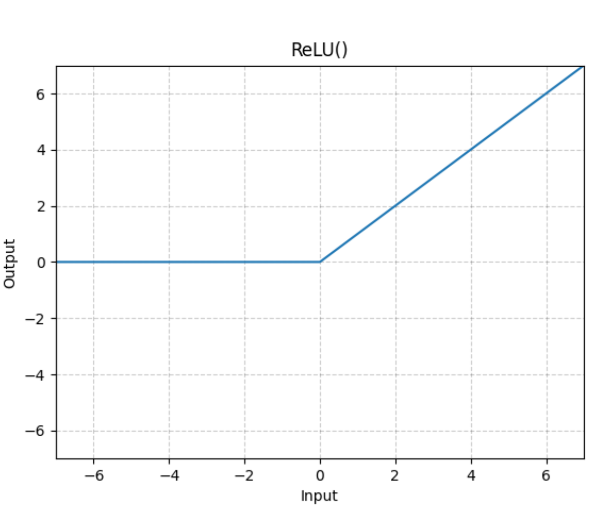
(1) ReLu(Rectified Linear Unit)
$$
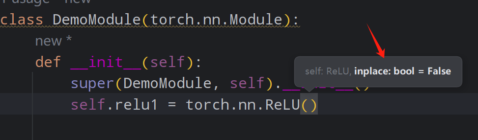
这个inplace(替换):
True:直接把变换后的值,放到input的那个变量里面
False:把变换后的值,需要一个新的变量来接收
1
2
3
4
5
6
7
8
9
10
11
12
13
14
15
16
import torch i = torch.tensor([[-1 , 2 , 3 ], [4 , -5 , 6 ], [7 , 8 , -9 ]]) i = torch.reshape(i,(-1 ,1 ,3 ,3 )) class DemoModule (torch.nn.Module): def __init__ (self ): super (DemoModule, self).__init__() self.relu1 = torch.nn.ReLU(inplace=False ) def forward (self, x ): return self.relu1(x) mod = DemoModule() output = mod(i) print (output)
(2)Sigmoid
$$
8.5 Linear model
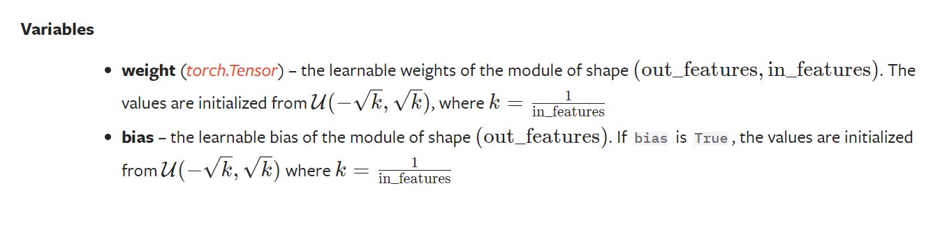
nn.Linear
in_features (int
out_features (int
bias (bool False, the layer will not learn an additive bias. Default: True
就是全连接层。把数据摊平 之后,进行kx+bias的变化,再输出到指定数目的节点去。
#torchflattentorch.flatten:把数据展开到一维
9 损失函数与反向传播
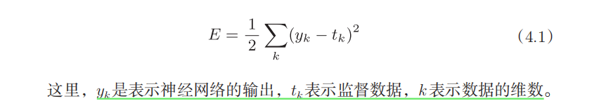
损失函数
神经网络通过学习损失函数(Loss Function) 寻找最优权重参数。
计算实际输出和目标之间的差距
为更新输出提供依据(反向传播),grad(梯度)
#损失函数
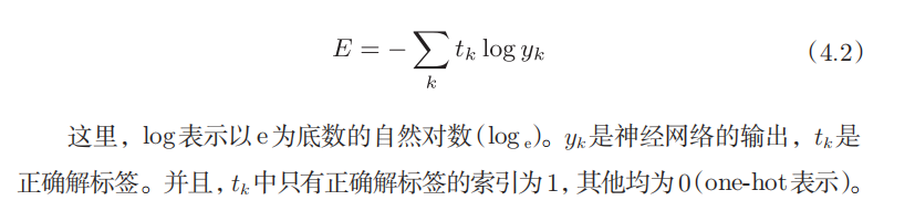
只计算对应正确解标签的输出的自然对数。
1
2
3
4
5
6
7
8
9
10
11
12
13
14
import torch.nn as nn import torch loss = nn.L1Loss() input = torch.randn(3 , 5 , requires_grad=True ) target = torch.randn(3 , 5 ) print (input ) print (target) output = loss(input , target) print (output) loss_mes = nn.MSELoss() result_mse = loss_mes(input , target) print (result_mse)
反向传播
10 优化器
#优化器
https://pytorch.org/docs/stable/optim.html
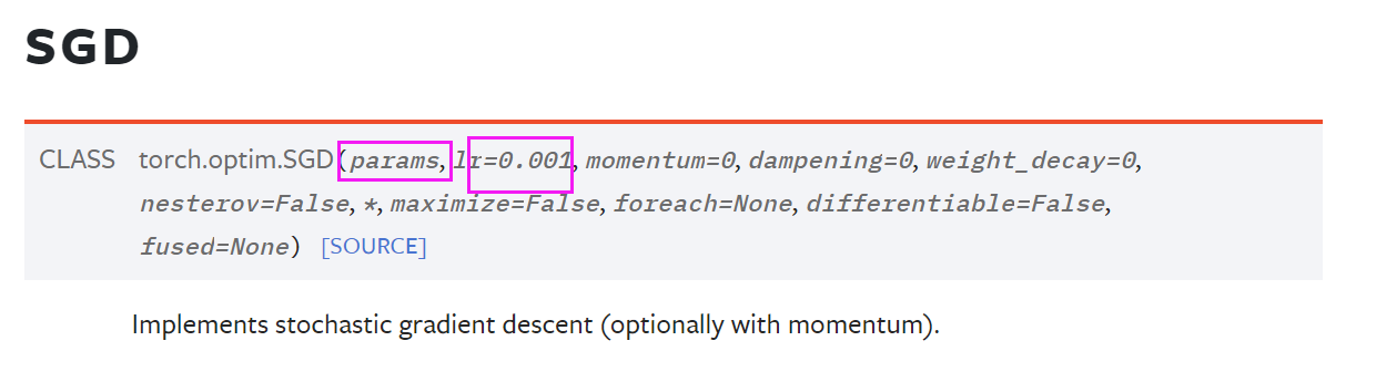
SGD随机梯度下降
#SGD
1
2
3
4
optimizer = optim.SGD(model.parameters(), lr=0.01 , momentum=0.9 ) optimizer = optim.Adam([var1, var2], lr=0.0001 )
初始化参数
1
2
3
4
optim.SGD([ {'params' : model.base.parameters(), 'lr' : 1e-2 }, {'params' : model.classifier.parameters()} ], lr=1e-3 , momentum=0.9 )
这里的代码使用了PyTorch中的optim.SGD优化器来训练模型。这个优化器采用了随机梯度下降(Stochastic Gradient Descent,SGD)的方法,并添加了动量(momentum)来加速训练过程。
具体解释如下:
optim.SGD : 这是一个优化器,它实现了随机梯度下降算法。SGD是一种常用的优化算法,用于调整模型参数以最小化损失函数。
params : 这里指定了要优化的参数集合。代码中将模型的参数分成了两组,分别设置了不同的学习率(learning rate,lr)。
{'params': model.base.parameters(), 'lr': 1e-2}:这表示模型的基础层(base)参数使用一个学习率为0.01(1e-2)的值进行优化。
{'params': model.classifier.parameters()}:这表示模型的分类器(classifier)层的参数。没有指定单独的学习率,因此这些参数将使用外层的学习率1e-3。
lr : 学习率是一个超参数,控制每次参数更新的步长。这里有两个学习率:
1e-2(0.01)用于基础层参数。1e-3(0.001)用于分类器层参数(外层指定的学习率)。
momentum : 动量是一个超参数,用于加速SGD在相关方向上的收敛,并抑制震荡。动量项在参数更新时引入了历史梯度的累积,使得优化过程更稳定。这里设置的动量值为0.9。
综上所述,这段代码的含义是使用带有动量的随机梯度下降算法来优化模型的参数,其中基础层参数的学习率设置为0.01,分类器层参数的学习率设置为0.001。动量参数设置为0.9。这样可以在训练过程中更好地控制模型的更新步长和收敛速度。
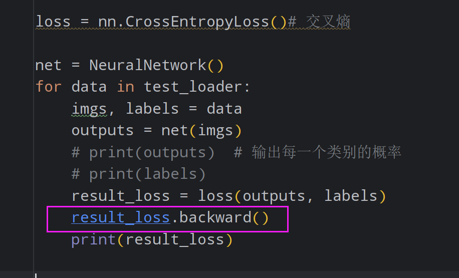
1
2
3
4
5
6
7
8
9
10
11
for input , target in dataset: optimizer.zero_grad() output = model(input ) loss = loss_fn(output, target) loss.backward() optimizer.step()
训练部分代码:
1
2
3
4
5
6
7
8
9
10
11
12
13
14
15
16
17
18
19
20
21
loss = nn.CrossEntropyLoss() net = NeuralNetwork() optimizer = torch.optim.SGD(net.parameters(), lr=0.01 ) for epoch in range (20 ): running_loss = 0.0 for data in test_loader: """ 这个for相当于只对data进行了一轮的学习, 通常需要好几轮的学习,才能有所改善。 所以需要外层的epoch """ imgs, labels = data outputs = net(imgs) result_loss = loss(outputs, labels) optimizer.zero_grad() result_loss.backward() optimizer.step() running_loss = running_loss + result_loss print ("epoch:{}, loss:{}" .format (epoch, running_loss))
11 现有网络模型的使用和修改
在pytorch的官方文档中,torchvision或torchtext等文件中,包含了相关领域中的经典网络模型。
11.1 VGG简介
常用的版本:
vgg16
pretrained:在ImageNet中与训练(这个数据集130G+,而且不能torchvision直接下载,需要自己寻找资源)
progress:下载进度条
vgg19
初始化的时候,True会下载参数(很大)
VGG16常被用来作为迁移学习等模型的前半部分,用于提取一些图像的特殊特征,在后续的模型中对这些特征进行一个进一步的学习。
利用现有的网络,套到自己的数据集上
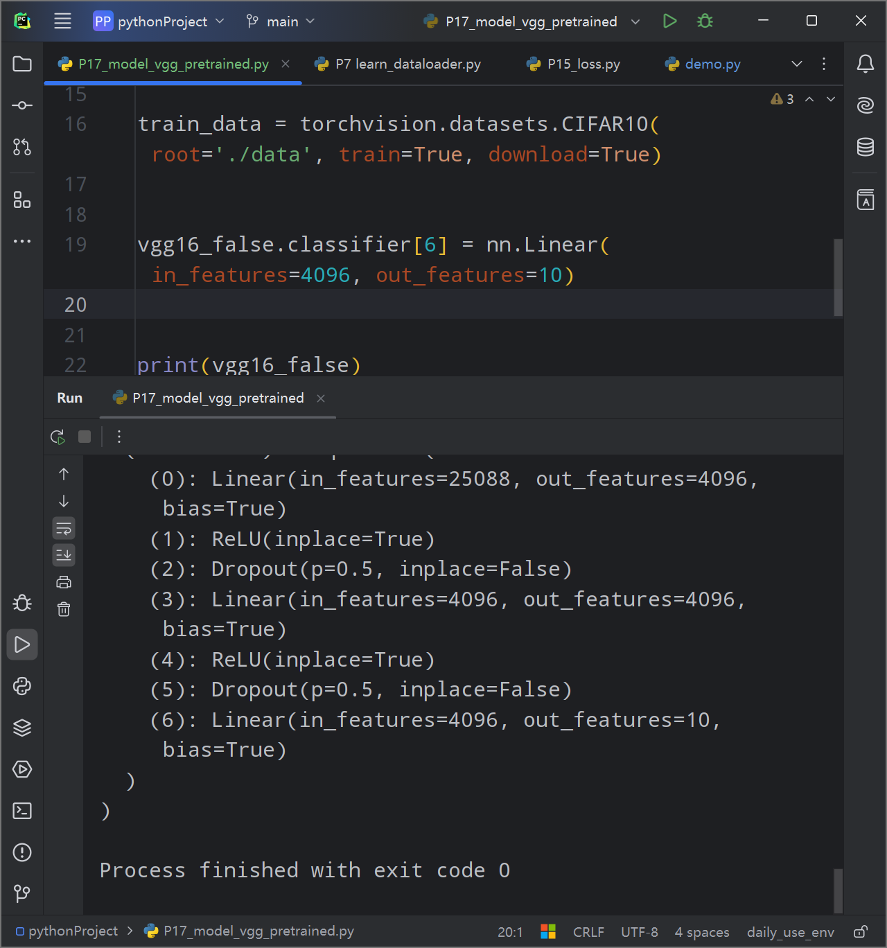
VGG使用了ImageNet进行训练,输出的最后一层与ImageNet的类别数量相同,都是1000,如何把这个现有的模型改成我需要的模型?
之前的数据集为例
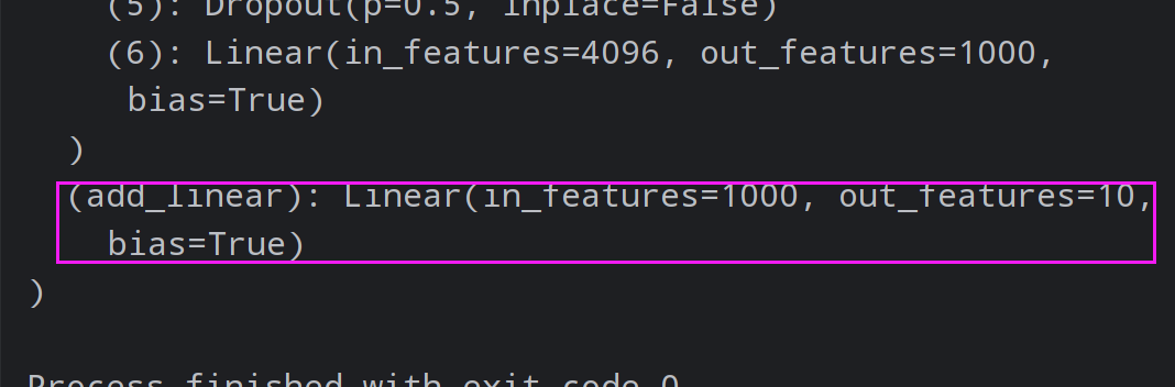
方法一:把最后一个输出层后追加一层input为10000,output为10的线性层。
1 vgg16_false.add_module('add_linear' , nn.Linear(1000 , 10 ))
如果要加到上面那个括号(classifier)里面:
1 vgg16_false.classifier.add_module('add_linear' , nn.Linear(1000 , 10 ))
12 网络模型的保存与读取
12.1 保存模型与参数
这种方法可以保存模型的结构和模型的参数。
若模型较大,则保存文件也会很大
Save model
1
2
vgg16 = torchvision.models.vgg16(pretrained=False ) torch.save(vgg16, 'vgg16_method.pth' )
第一个参数:模型
1 2 model_1 = torch.load("vgg16_method.pth" )
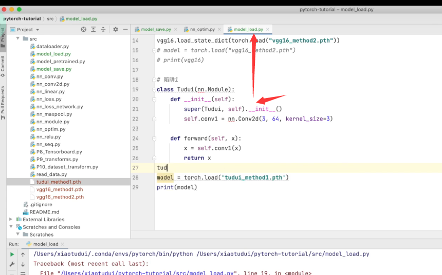
这个方式是存在陷阱的:
为了解决这个问题,则需要自己重新定义一次自定义的模型结构:
比如我在model文件创建并保存了数据,在load文件里面需要重新定义(无需new)一次这个模型,才能继续正常使用
12.2 保存模型参数
这个方法将模型的参数作为字典进行保存,所以加载的时候,要用字典加载的方式,放入新的模型中。
官方推荐的方法
1 torch.save(vgg16.state_dict(), 'vgg16_state_dict.pth' )
1 2 3 4 5 6 7 8 9 10 PATH = "state_dict_model.pt" torch.save(net.state_dict(), PATH) model = Net() model.load_state_dict(torch.load(PATH)) model.eval ()
[!NOTE]
12 完整模型训练套路
以CIFAR10 为例
步骤说明:
初始化训练集、测试集,转换为Dataloader
初始化自己的模型
定义损失函数和优化器
定义训练次数 epoch
进行迭代epoch
从dataloader中每次取数据进行训练
得到output
得到output与labels的loss
优化器置零
反传播
优化器优化参数
在测试集中检测——取消grad
在流程中合适的地方对结果进行输出或者保存。
定义模型
1
2
3
4
5
6
7
8
9
10
11
12
13
14
15
16
17
18
19
20
21
22
23
24
25
26
27
28
29
30
31
32
33
34
35
36
''' @Project :pythonProject @File :MyModel.py @IDE :PyCharm @Author :周大猛 @Date :2024/05/20 15:21 ''' import torch from torch import nn class TongModel (nn.Module): def __init__ (self ): super (TongModel, self).__init__() self.model = nn.Sequential( nn.Conv2d(3 , 32 , kernel_size=5 , stride=1 , padding=2 ), nn.MaxPool2d(2 ), nn.Conv2d(32 , 32 , 5 , 1 , 2 ), nn.MaxPool2d(2 ), nn.Conv2d(32 , 64 , 5 , 1 , 2 ), nn.MaxPool2d(2 ), nn.Flatten(), nn.Linear(64 * 4 * 4 , 64 ), nn.Linear(64 , 10 ), ) def forward (self, x ): x = self.model(x) return x if __name__ == '__main__' : model = TongModel() input = torch.ones((64 , 3 , 32 , 32 )) output = model(input ) print (output.shape)
[!NOTE]
数据集
1 2 3 4 5 6 7 8 9 10 11 12 13 14 15 train_data = torchvision.datasets.CIFAR10(root='./data' , train=True , download=True ,transform=transforms.ToTensor()) test_data = torchvision.datasets.CIFAR10(root='./data' , train=False , download=True ,transform=transforms.ToTensor()) train_data_size = len (train_data) test_data_size = len (test_data) print ("Train data size: {}" .format (train_data_size) ) print ("Test data size: %d" % test_data_size) train_dataloader = DataLoader(train_data, batch_size=64 , shuffle=True ) test_dataloader = DataLoader(test_data, batch_size=64 , shuffle=True )
[!NOTE]
导入神经网络,初始化模型
模型初始化
损失函数
优化器
学习率
训练进度
测试进度
迭代次数
保存数据位置
1
2
3
4
5
6
7
8
9
10
11
12
13
14
15
16
17
from MyModel import * model = TongModel() loss_fn = nn.CrossEntropyLoss() learning_rate = 1e-2 optimizer = optim.SGD(model.parameters(), lr=learning_rate, momentum=0.9 , weight_decay=5e-4 ) total_train_step = 0 total_test_step = 0 epoch = 100 writer = SummaryWriter('./logs_train' )
训练与测试
1
2
3
4
5
6
7
8
9
10
11
12
13
14
15
16
17
18
19
20
21
22
23
24
25
26
27
28
29
30
31
32
33
34
35
36
37
38
39
40
41
42
43
44
45
46
47
for i in range (epoch): print ('Epoch {}/{}' .format (i, epoch)) model.train() for data in train_dataloader: imgs, labels = data output = model(imgs) loss = loss_fn(output, labels) optimizer.zero_grad() loss.backward() optimizer.step() total_train_step += 1 if total_train_step % 100 == 0 : print ('Total train step:{}, Loss:{}' .format (total_train_step, loss.item())) writer.add_scalar('Loss/train' , loss.item(), total_train_step) """ 每次训练一轮之后,需要知道本次训练之后在测试集上模型表现是否有进步。 在第一层的for中,对此进行检测。 这里不需要对模型进行调优。 需要知道在整个数据集上的loss """ model.eval () total_test_loss = 0.0 total_accuracy = 0 with torch.no_grad(): for data in test_dataloader: imgs, labels = data output = model(imgs) loss = loss_fn(output, labels) total_test_step += 1 total_test_loss += loss.item() accuracy = (output.argmax(dim=1 )==labels).sum () total_accuracy += accuracy.item() print ('Total test Loss:{}' .format (total_test_loss)) writer.add_scalar('Loss/test' , total_test_loss, total_test_step) print ("整体测试集的正确率:{}" .format (total_accuracy/test_data_size)) writer.add_scalar('Accuracy/test' , total_accuracy/test_data_size, total_test_step) torch.save(model.state_dict(), './modelData/model_{}.pt' .format (i)) writer.close()
13 使用GPU训练
有两种使用GPU的方式
13.1
.cuda
1 2 3 model = TongModel() model = model.cuda()
在训练和测试的部分
1
2
3
imgs, labels = data imgs = imgs.cuda() labels = labels.cuda()
1 2 3 loss_fn = nn.CrossEntropyLoss() loss_fn = loss_fn.cuda()
良好的写法:
13.2
方法二:.to(device)
定义训练的设备1 2 device = torch.device('cuda' if torch.cuda.is_available() else 'cpu' )
然后之前该国的地方都改成
14 完整模型验证套路
给训练好的模型提供输入。
与测试部分类似,大概流程如下:
准备数据(自己准备的,非数据集的测试部分或训练部分)
导入模型
模型初始化
模型参数初始化
在测试模式下,输入准备的数据
获得结果,并进行对比
15 Github开源代码
只说说注意事项:
仔细阅读README
参数部分可以在代码中找到描述